Introduction
Thanks a bunch for the quick and concise reply! I took some days to go through the linked post, followed by the forum in general. Still digesting all the information, but I figured I would write some of my thoughts down while they’re still fresh, with the slight chance that it might be of interest to some in the community. Apologies if it is not, and worst case I’m thankful for a place to order some of my own confusion  .
.
I’m a computer scientist by trade, so my point of view is one of the student, tipping his toes into an exciting new field. It will also be highly subjective at points, so absolutely feel free to disagree!
Kind of a tl;dr at the end.
About the Dual
The concept of duality is such a beautiful one. In the context of GA (and PGA specifically) however it seems to be frequent cause for both confusion among newcomers as well as discussion among experts. The by now infamous thread about why use dual space in PGA was, as @bellinterlab puts it, “quite enlightening”.
So I started out by trying to understand the various concepts, from Poincaré and Dual maps to Hodge Duals and Reciprocal Frames. Followed by quite the adventure to figure out some of the missing puzzle pieces and gaps, including the choice of basis and how to actually compute the dual.
At this point I had already done some very intriguing experiments using ganja.js, where mocking up a 2D-shadow caster using PGA is just such a fun project to get started!
\mathbb{R}_{2,0,1} and the available implementations is a great starting point for newbies.
However, I hit a wall of understanding, with some unanswered questions lingering in my head. So I decided to sit down and start from scratch, drawing some pretty Cayley tables and deriving some of the operations by hand.
The following outlines some of my findings and conclusions of these early adventures.
The Choice of Basis
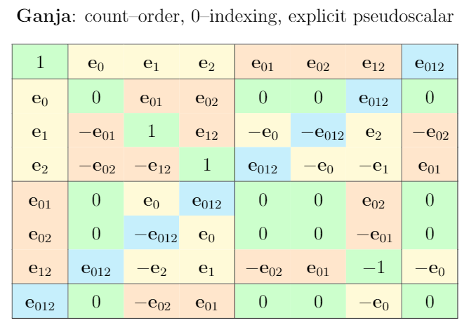
The first time I stumbled upon the topic was related to ganja.js, which uses \mathbf{e}_{02} instead of \mathbf{e}_{20}, allegedly in order to account for the Y-down orientation in 2D-rendering. I soon came to realize though that the implications of how we name, write and order our basis vectors and blades go much deeper.
Notation
The first point I want to make highlights two aspects in particular, both of which are of somewhat subjective nature.
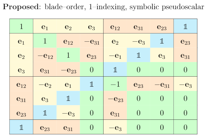
0-indexing vs. 1-indexing
For me, starting e.g. from two basis vectors \mathbf{e}_1, \mathbf{e}_2 \in \mathbb{R}_{2,0,1}, it felt more natural to add the additional 1-up dimension at the end, rather than at the front, i.e. introduce \mathbf{e}_3 rather than \mathbf{e}_0. I likely have been primed this way during my studies and career, but looking at Cayley tables with \mathbf{e}_0 in the first column feels “off” to me. Maybe also due to the fact that all my math courses in university used 1-indexing.
More objectively, an argument I’ve seen being made in favor of 0-indexing is that the translational element stays consistent in all dimensions. I find this argument can be flipped though, noticing that vice-versa the basis always starts with the “bulk” of the object using 1-indexing.
In practice, I’d assume that a slight majority of enthusiasts would be more comfortable with 1-indexing for basis vectors, lowering the bar for cross-discipline beginners. This is of course speculative, it was at least true for myself.
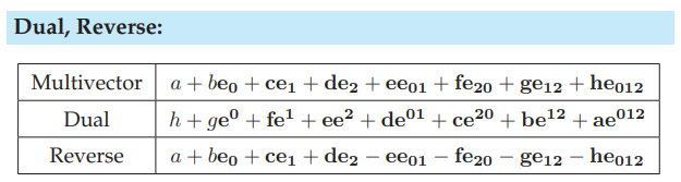
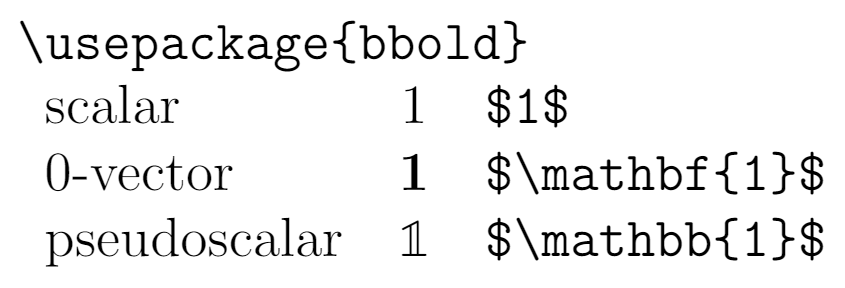
Pseudoscalar Symbol
A second aspect is a notational one, concerning the pseudoscalar. In written form, it’s often denoted by I. In calculations and tables, it’s often being written in terms of its basis vectors, e.g. \mathbf{e}_{1234}. This clutters formulas and tables alike, especially in higher dimensions.
There’s an alternative notation, that I’ve first seen in @elengyel’s work, who uses blackboard boldface \mathbb{1} instead. I got to like this notation a lot and hope to further advocate its adoption in the GA community, in both paragraph and table context.
Side-by-Side Comparison
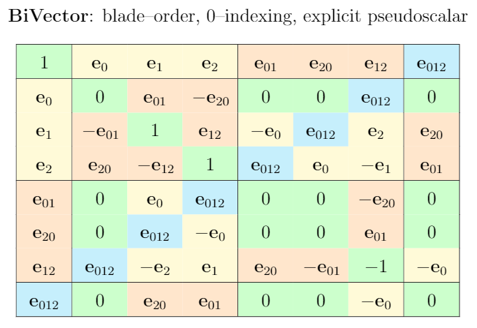
I drew up the Cayley tables for \mathbb{R}_{2,0,1} as defined by ganja.js, biVector, as well as my own favorite form, respectively.
Complements
This is where it got interesting. Drawing up my first \mathbb{R}_{2,0,1} Cayley tables, I noticed that both the order of blades, but more significantly the order of basis vectors that define those blades has implications reaching farther than I was yet aware of.
Oder of Blades
Rather obvious - but still something I needed to discover first - is the fact that by simply arranging blades in one way or another, it is possible to shape the table’s anti-diagonal.
For any PGA Cayley table, it is possible to arrange the blades in such a way that the anti-diagonal items result in \pm\mathbb{1}.
Order of Basis Vectors
Similarly, we can influence the sign of pseudoscalars on the anti-diagonal by swapping the order in which we multiply basis vectors. As mentioned before, there is for example a discrepancy in the biVector cheat sheet and the ganja.js implementation, where the latter has -\mathbb{1} on some of its anti-diagonal elements. In this case, it was likely just an implementation detail, and doesn’t really matter, but for educational purposes, I would argue that having
non-negative pseudoscalars on the anti-diagonal is desirable.
And apart from simplicity and visuals, there are mathematical implications I’ll get into in the next section.
While for \mathbb{R}_{2,0,1} it is rather simple to find such an ordering, it is impossible to do so in \mathbb{R}_{3,0,1}. Consider for example \mathbf{e}_{234} \wedge \mathbf{e}_{1}. The vector-element needs to swap places three times to get it to the front and form \mathbf{e}_{1234}, no matter what. There’s simply no way around it! This inherently introduces the negation due to anti-commutativity. @enki already notes, that in a choice for a proper basis, the minus signs are on the trivectors, e.g. similar to the biVector cheat sheet.
1, \mathbf{e}_{0}, \mathbf{e}_{1}, \mathbf{e}_{2}, \mathbf{e}_{3}, \mathbf{e}_{01}, \mathbf{e}_{02}, \mathbf{e}_{03}, \mathbf{e}_{12}, \mathbf{e}_{31}, \mathbf{e}_{23}, \mathbf{e}_{021}, \mathbf{e}_{013}, \mathbf{e}_{032}, \mathbf{e}_{123}, \mathbb{1}
This property is imo due to the axioms of the complement, which @chakravala mentions here. While I agree that this forms a “nicer” basis, @elengyel on his poster chose an order such that both tri- and bivector pseudoscalar become negated.
1, \mathbf{e}_1, \mathbf{e}_2, \mathbf{e}_3, \mathbf{e}_4, \mathbf{e}_{23}, \mathbf{e}_{31}, \mathbf{e}_{12}, \mathbf{e}_{43}, \mathbf{e}_{42}, \mathbf{e}_{41}, \mathbf{e}_{321}, \mathbf{e}_{124}, \mathbf{e}_{314}, \mathbf{e}_{234}, \mathbb{1}
Curious as to why that choice has been made! All of this however led me to the discovery I made next.
The Great Collapse.
For the math-savvy here this is old news, but I made a small jump when I discovered the connection between basis ordering and the complement operators. To recap - and this is only my understanding at this point - the (some™)
dual operator generalizes to a left- and right-complement.
Bluntly put, they flip the coefficients of the current base, and sometimes have some seemingly magic sign flips in there as well, just for good measure. However, the revelation for me was to realize that the sign directly correlates with the Cayley table’s anti-diagonal, which in turn led me to finally make the cognitive connection between blades and their duals. In some spaces, the complements inherently “flip” as is the case in \mathbb{R}_{3,0,1} as described above for all trivectors. The complement operator of course mirrors this behavior by flipping the sign on the according coordinates to generate a proper dual representation over the same basis.
I was confused for quite a while why Eric’s poster kinda had two dual operators, left- and right-complement. With the new found understanding, this finally made sense and also helped me understand the necessity for both J and J^{-1} and similar in other models. Now, here comes the part where my mind got blown. In \mathbb{R}_{2,0,1} (and by extension generally any odd-dimensional geometric algebra), due to the fact that the anti-diagonal can be constructed completely non-negative, the left- and right-complements collapse to a single dual operator!
lc(a) = rc(a), a \in \mathbb{R}_{n_-,n_+,n_0} \Leftrightarrow (n_- + n_+ + n_0) \in (2 \mathbb{Z} + 1)
I don’t have the mathematical prowess to prove this claim. It just feels right and somewhat intuitive to me. Glad if anyone can chime in with comments or references, this is likely no news at all, some good paper to read maybe?
As a last comment on this, it seems to me that choosing a basis with as few negations as possible would also benefit GA implementations, minimizing operations. It would be interesting to see what influence the choice of basis has on common GA operations like join, meet, project etc. themselves - if any. Maybe after factorizing everything out, it’s just as many ops (additions, multiplications) one way or the other?
Where to Next
Thanks for reading so far! Some closing thoughts and tl;dr.
Curriculum
I only got into GA recently, and it’s been a lot of fun and excitement. In hindsight, I have a couple suggestions on what helped me at least to understand and get a better grasp on things.
2D PGA is a Great Starting Point
- The projective aspect can still be visualized and conceptualized by our minds in 3D
- Cayley tables behave nicely, not much ambiguation to figure out
- The left- and right-complements collapse to a single dual operation
- Coding up some fun examples is straight forward and very rewarding!
The Move to 3D PGA
- Use Cayley table to intuitively illustrate complement “flip”
- Introduce left- and right-complement as generalized dual operator
- Outline both geometric product, wedge and their dual operators
Blackboard Boldface Pseudoscalar
- It’s the way to go

- Improves readability of calculations and tables
- Simply fun to write
Personal Agenda
Things I want to do next.
Open Questions
- Is the whole complement-collapse idea correct in the first place?
- Does it in fact hold for odd-dimensional algebras?
- What are further implications of choice of basis, e.g. on implementation performance?
2D PGA Duality Cheat Sheet
- Introduce dual operators with in beginner-friendly 2D PGA setting
- Side-by-side comparison of common formulas and their duals
- Collaboration welcome!
2D PGA Applications
- Already working on a fun little browser game
- Looking into implementing primal-based implementation using dual geometric product
Conclusion
Thank you if you actually took the time, effort and patience to crunch through this wall of text! Hope it was at least an interesting insight into the experience of learning GA from my outside perspective, if nothing else.
Cheers and all the best!