Reflection at parabola with GA

[Egbert]

Hello!

I’m 1/2 year into GA now, amazed, overwhelmed, confused (GA, PGA, CGA?). GA highly inspires me, and besides Infinitesimals/Hyperreal Numbers/Surreal Numbers, it is one of the things in Math that I always missed in school and university, that just felt like it had to be there, but noone could tell or point to; and that I finally found.

I could think of a gazillion problems that seem to be easy with or lending themselves to GA, but as a starter I want to tackle a single problem to learn to do “real” problems with GA.

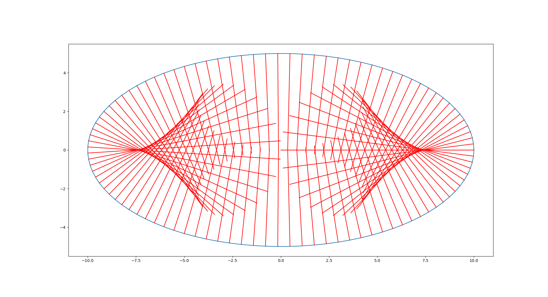
I wonder how one would model the reflection of lines going through a point (“source”) at a parabola.

First I would like to solve the the obvious case: Source at focus of the parabola.

Then I’d like to look into other source points, going on with other curves that act as reflector. Then I’d like to look into the “density” of lines, and even something like incidence angle (at an intersection), occlusion (Heaviside function), variation of parameters, 3D case…

Uses could be modeling a lamp like a Poul Henningsen PH 5, or a Wolter telescope.

Things where I am stuck/unsure and need help:

• Which GA is best suited (for the 2D case, later maybe 3D)
• How do I describe a curve or function in GA? Parabola, standard form, rotation?
• How do reflect at a curve? Would of course need the tangent at the point of reflection…
• The source is a pencil of lines, which has a known representation in some GA’s, and if it is at the focus of the parabola, the outcome has to be a pencil of lines though some point at infinity (parallel) lines. But I’m not sure if the density is uniform, and how to analyse that. Of course in a more general case the outcome is more complicated.
• How do I analyse/model different densities of pencils?

Any pointers to papers, videos, presentation, books etc. are highly welcome, along of course explanations of actual steps.

I find tons of theoretic material regarding basics and properties of GA, but miss the actual practical examples.

[cgunn3]

@Egbert This is an interesting question!

I think that 2D euclidean PGA is a good tool for solving it.

I’ve written a ganja demo that carries out the reflection of a line pencil in a parabola in this context.

Here’ll I’ll give a sketch of the ideas behind the code. You can look at the source code for the details.

For simplicity assume the parabola C is the standard one y = x^2. Parametrize it as C(t) = e_{12} + t e_{20} + t^2 e_{01}. For future reference, compute the derivative \dot{C}(t) = e_{20} + 2t e_{01}.

Let m be a line in the line pencil centered at P (or "the line pencil in P"). Let M be an intersection of m with C. Given M, it is easy to find the unique t satisfying C(t) = M. Then the tangent line t_M at M is given by the join of the point with the direction of movement at the point: t_M = C(t) \vee \dot{C}(t) (= -2t e_{1} + e_2 + t^2 e_{0}).

With t_M in hand, the reflection of m in t_M is given by the sandwich t_M m t_M, and ganja does the rest.

[cgunn3]

June 7, 2021: I’ve added color coding to the demo. Each line in the pencil is assigned a color between red and blue. Then the geometry associated to that line (intersection points with parabola, their tangent lines, and the reflected lines) are drawn with the same color.

In general, such a reflected line pencil is called a caustic curve with respect to the reflecting curve. This curve is naturally in line-wise form (as described above). But like every well-behaved curve, it also has a point-wise form. I’ve implemented an approximation to this point-wise caustic, obtained by intersecting consecutive lines of the line-wise caustic. The exact point-wise curve is obtained by the wedge product r(t) \wedge \dot{r}(t) where r(t) is the line-wise form. In general r(t) \wedge \dot{r}(t) is the instantaneous center of rotation of a line-wise curve r(t), just as C(t) \vee \dot{C}(t) is the instantaneous line of motion of a point-wise curve C(t).)

Exercise: Use the automatic differentiation feature of euclidean PGA to replace the approximate caustic curve with the exact caustic curve.

[joha2]

@cgunn3 Thank you very much for your explanations on that matter! This helped me a lot to get an idea how to use PGA in a more differential geometric setting (like derivatives of curves, tangents, and so on) and also how to generalize this to surfaces (like for z = f(x, y) which is described pointwise via p = e_{123} + x e_{032} + y e_{013} + f(x, y) e_{021}, the tangent plane in a certain point is given by T = p \wedge \partial_x p \wedge \partial_y p).

There is one question, which crossed my mind: For describing curves/surfaces this way, we always need an explicit formulation of the coordinates. Is it possible to describe also implicit functions like F(x, y, z) = 0 in a nice PGA manner? I mean, the obvious one is: use a point p = e_{123} + x e_{032} + y e_{013} + z e_{021} such that for all x, y, z the equation F(x, y, z) = 0 is fulfilled. But this is not very appealing . And connected to this: Is there a nice formulation for quadrics, like its matrix formulation (\bold{x}, 1)^T\,A\,(\bold{x}, 1) = 0, where A is a 4\times 4 matrix? Thanks again!

Best wishes
Johannes

[cgunn3]

@joha2 I’m glad you could learn something useful from this example.

Regarding your questions, I’m afraid I can’t offer any geometric algebra advantages besides general ones.

Implicit functions f(x,y,z) = 0 seem fundamentally hard. In PGA there are neat tricks to be played by being able to consider the level surfaces as either point-wise or plane-wise (just as in the parabola example you move back and forth between point-wise and line-wise curves) and perhaps that can provide a more agreeable infrastructure, but I don’t see any help for actually solving the implicit equation.

Regarding quadric surfaces: PGA is based on a special quadric, the so-called absolute, that is determined by the signature, for example (2,1,0) (the hyperbolic plane) is the quadric x^2 + y^2 -z^2 = 0. The points lying on this quadric are the so-called ideal (or null) points of the Cayley-Klein space and have 0 norm. Multiplying by the pseudoscalar carries out the “polarity” on this quadric, which maps every subspace to its orthogonal subspace …

But that doesn’t really help if you’re interested in another quadric Q (represented by a symmetric matrix B). I would recommend representing it as a so-called “outermorphism” of the algebra. Essentially, Q can be thought of as defined on the vector space of 1-vectors; there are canonical methods to obtain the induced matrices for the higher rank vector spaces of k-vectors. A full-fledged GA package should provide support for that, or look at this wikipedia article on outermorphisms.

Sorry I can’t be more encouraging; perhaps there are others in the community who know better.

[joha2]

Hey @cgunn3! Thanks for your fast response! First of all, I made a mistake above: It has to be T = p \vee \partial_x p \vee \partial_y p of course. Maybe there are others . I also did not find the button to edit my comment.

How does this playing around with level surfaces work? I can only imagine to find some explicit form of f(x, y, z) = 0 when some of the entries are fixed (say e.g. for f(x, y, z_0) = 0). Or is there a possibility to use something like the theorem about implicit functions for PGA?

About the quadrics: Yeah I understand your point. Let’s say I have a 3\times3 matrix A, than this represents some linear map A:\mathbb{R}^3 \to \mathbb{R}^3 such that {\bf e}_i \cdot A({\bf e}_j) = A_{ij}. This could be generalized to higher rank k-vectors via outermorphism. From this I could imagine to extend e.g. a centered ellipsoid to bivectors in \mathbb{R}^3. But in PGA I have several problems here:

• Vectors describe planes, not points (ok they are dual to each other ).
• {\bf e}_0 \cdot {\bf e}_0 = 0 (this cuts of some components in higher powers).
• I see no way to form “higher powers” of points.

I would have thought that the description of a quadric in homogenious coordinates ({\bf x}, 1)^T A ({\bf x}, 1) = 0 is somehow compatible with PGA, but even if we say, let’s “translate” this by using something like p^\ast \cdot A(p^\ast) = 0, we lose some components due to {\bf e}_0 \cdot {\bf e}_0 = 0. But maybe PGA is more or less restricted to linear structures which it describes very well and for nonlinear ones, one has to use other GAs.

Best wishes
Johannes

[cgunn3]

The outermorphism is defined only in terms of the non-metric operations of PGA (i. e. the outer product). The inner product plays no role. As the Wikipedia article on the subject mentions at the beginning, the outermorphism is defined on the exterior algebra (which is essentially the geometric algebra with the metric removed). I hope to have time to write this up in a bit more detail with special attention to the case where the matrix Q represents a quadric surface (i. e., is symmetric and full rank).

[joha2]

Thanks for the clarification! Yes, the scalar product in the formula above is unnecessary, maybe it is better to use A({\bf e}_i) = \sum_j A_{ij} {\bf e}_j which is without any metric reference. When I use the outermorphism property, I get e.g. A({\bf e}_i \wedge {\bf e}_j) = A({\bf e}_i) \wedge A({\bf e}_j) = \sum_{k\ell} A_{ik} A_{j\ell} {\bf e}_k \wedge {\bf e}_\ell, which has also no metric reference. Is this correct so far? Although, for me, it is not clear how to use this for a quadric in PGA Thanks for writing this down!

[joha2]

I found a solution: Let x be the point which is given by x = ({\bf e}_0 + {\bf x})^\ast. Then x \wedge x^\ast = (1 + {\bf x}^2) I. Now one can use a linear map A, which is defined by A({\bf e}_0) = A_{00} {\bf e}_0 + \sum_i A_{i0} {\bf e}_i and A({\bf e}_i) = A_{0i} {\bf e}_0 + \sum_j A_{ji} {\bf e}_j and apply it to the right hand side of the wedge product above. x \wedge A(x^\ast) = (A_{00} + \sum_i (A_{0i} + A_{i0}) x_i + \sum_{ij} A_{ij} x_i x_j)I which corresponds to ({\bf x}, 1) \mathcal{A} ({\bf x}, 1)^T above (the 0 corresponds to the position of the 1 in the vector, \mathcal{A} is the matrix for the linear map A) and is totally free of some metric (if \ast is free of metric ). x_i denote the components of the vector {\bf x}.

The only thing what is missing for my understanding is some kind of geometrical meaning: in the case of x\wedge P = 0 where P is some plane, one checks whether x lies in the plane P. But here x is related to its dual plane x^\ast … strange.

Best wishes
Johannes

[joha2]

I also observed, that if one uses the geometric product x\,x^\ast (or xA(x^\ast)) then setting the I part constant leads to a quadric surface and using the same variables (i.e. \bold{x}) where c is constant on the arising “dual bivector” part of the geometric product gives the normal lines at this position on the quadric surface for free. At the end the positions on the quadric surface have to be calculated via solving well known algebraic equations, but the normals are provided for free without calculating derivatives and so on. That’s nice!

Here I drew the points where the I part is constant in blue and the vector part of the geometric product from the points on the ellipse to their shortest distance to the origin in red.

[cgunn3]

It took me a while to realize what you were doing with the geometric product xx^*. You are getting the inner product \mathbf{x}\cdot \mathbf{x} this way, which isn’t accessible in the euclidean metric. And applying a symmetric A in the middle xA(x^*) gives you an arbitrary quadratic form Q(\mathbf{x}).

Now I have two questions regarding this post:

• Are you working in the plane (i. e., in 2D euclidean PGA), hence producing conic sections?
• Can you please write out more explicitly how you are producing the red normals? I don’t understand what ‘the arising “dual bivector” part of the geometric product’ means.

Thanks.

[joha2]

@cgunn3 thanks for your questions! I’ll try to answer them properly:

• Yes, for the picture above I used 2D euclidean PGA. In fact my hope was to produce conic sections and it looks like, the given recipe is at least a possibility to describe them in PGA.
• I borrowed the term ‘dual bivector’ from Leo from his series of talks together with Steven at SIBGRAPI . If x is a point, it is an n-vector in n-D PGA. Therefore x^\ast is a 1-vector, which means that their geometric product x\,x^\ast contains an n+1-vector part (proportional to I) and an n-1-vector part (called ‘dual bivector’ by Leo) which represents a line. The same argument holds for x\,A(x^\ast) since A maps 1-vectors to 1-vectors. For the product x x^\ast in 2D euclidean PGA one gets x\,x^\ast = (1 + x_1^2 + x_2^2) e_{012} + x_2 \bold{e}_1 - x_1 \bold{e}_2, where x_1, x_2 denote the point coordinates. For the ellipses the expressions are a little more complicated, but they lead to the red lines in the picture. As far as I understood, from the arguments given above, the recipe for the conic sections is not limited to 2D, but can also be used in higher dimensions.

I hope all is correct. If I made some mistakes, please tell me. I have a question, too: What do you mean by ‘the inner product is not accessible in the euclidean metric’? I also did not really understand, which role the metric of the underlying PGA plays here, since the I part is generated by an outer product, which is - as far as I understood - without any relation to the metric. Or is the metric introduced by the dual operation?

[joha2]

Coming back to the reflection of the parabola: Nearly all the given operations can be generalized to 3D without any head aches (i.e. formulation of the parabola, calculation of the tangential plane at the ray intersection, reflection of the incoming ray). What bothers me is the question: Is there any possibility to generalize the calculation of the caustic curve, too? At the end, the reflected rays are lines where I see no possibility to get to a plane or point description of some surface. Further, the intersection point depends on x and y and therefore also the reflected rays, so which parameter is used for the derivative which corresponds to \dot{r}(t)? Sorry for maybe a silly question

[cgunn3]

Hi @joha2
This is an interesting question!
Now we are taking a line bundle (all lines through a point) and reflecting it in the paraboloid.
When the point is at the focus, the image is a parallel line family, the bundle in the ideal point of the axis of the paraboloid.
When the point moves away from the focus but stays on the axis of the paraboloid, symmetry implies that the resulting caustic surface is obtained by rotating the corresponding 2D caustic curve around the axis. I think so anyway .
But for a point in general position, I don’t see how to proceed. I’ll think about it .

[joha2]

@cgunn3 Nearly one year later, I found (perhaps) an answer to the question of the caustic in 3D. As we already know, the parametrization of the parabola, the calculation of the rays and their reflections are straight forward: The point on the parabola is given by P(x, y) = O + x P_x + y P_y + \frac{x^2 + y^2}{2 R} P_z (O = e_{123}, P_x = e_{023} and so on), the source point is given by S = O + {\bf s} I and the ray is given by r(x, y) = S\vee P(x, y). The tangential plane at P is {\bf t} = P\vee P_{,x} \vee P_{,y}. Now we can calculate the reflected ray r^\prime = {\bf t} r {\bf t} as you mentioned above. (Btw: one of the insights for me was, that reflecting the ray is the same as reflecting the source and connecting reflected source and P ). Anyway: now, we can calculate the derivatives of r^\prime in x and y direction r^\prime_{,x} and r^\prime_{,y}. From these rays we can build up another ray via the commutator product c = r^\prime_{,x} \times r^\prime_{,y} which seems to be the caustic we are after. I calculated two test cases:

• I shifted the source to infinity S = {\bf s}I and let {\bf s} only have a z component: The result was a c which for all x, y intersected each other at the focal point at z = R/2 (tested by a plane with variable z-position and calculating the intersection with c). This is something, we would expect.
• The other case was: Setting S = O + {\bf s}I directly into the focal point at x = y = 0 and z = R/2. From this I got a c with only e_{0x} and e_{0y} components. As far as I understood, this is a line at infinity, but I don’t have a good geometric intuition for it. (Maybe you could help here.)

My questions are:

• Is there a simple explanation, why we use r\wedge \dot{r} for the point representation in 2D and r_{,x} \times r_{,y} for the line representation in 3D? It seems like, that the caustic is not easy generalizable to higher dimensions.
• Now we have probably a representation for caustic lines c(x, y). How to come from there to a point or plane representation of this surface? I can imagine that there has to be some sort of integrability condition. Are the c(x, y) tangential with respect to the desired surface? (OK, at the focal point there cannot be a surface representation and for the case of the source at the focal point I can also not see how to represent this as a surface. But for some non-extreme cases? Something like the curve r\wedge\dot{r}?)

Best wishes
Johannes